Tidy filtering, mapping and plotting in iso2k

Nick McKay

2024-09-11

LiPD filtering and mapping

library(lipdR)
library(geoChronR)
library(ggplot2)
library(magrittr)
library(dplyr)
library(purrr)

This vignette highlights how to filter, plot and map a library of LiPD data, but this time using the tidyverse framework. As before first let’s load version 1.0.0 of the iso2k database. Check out the details of the iso2k dataset Earth System Science Data.

iso <- readLipd("http://lipdverse.org/iso2k/1_0_0/iso2k1_0_0.zip")

That was easy - note that readLipd() can take individual LiPD files (ending in .lpd), or zip files full of LiPD files, directly from the web.

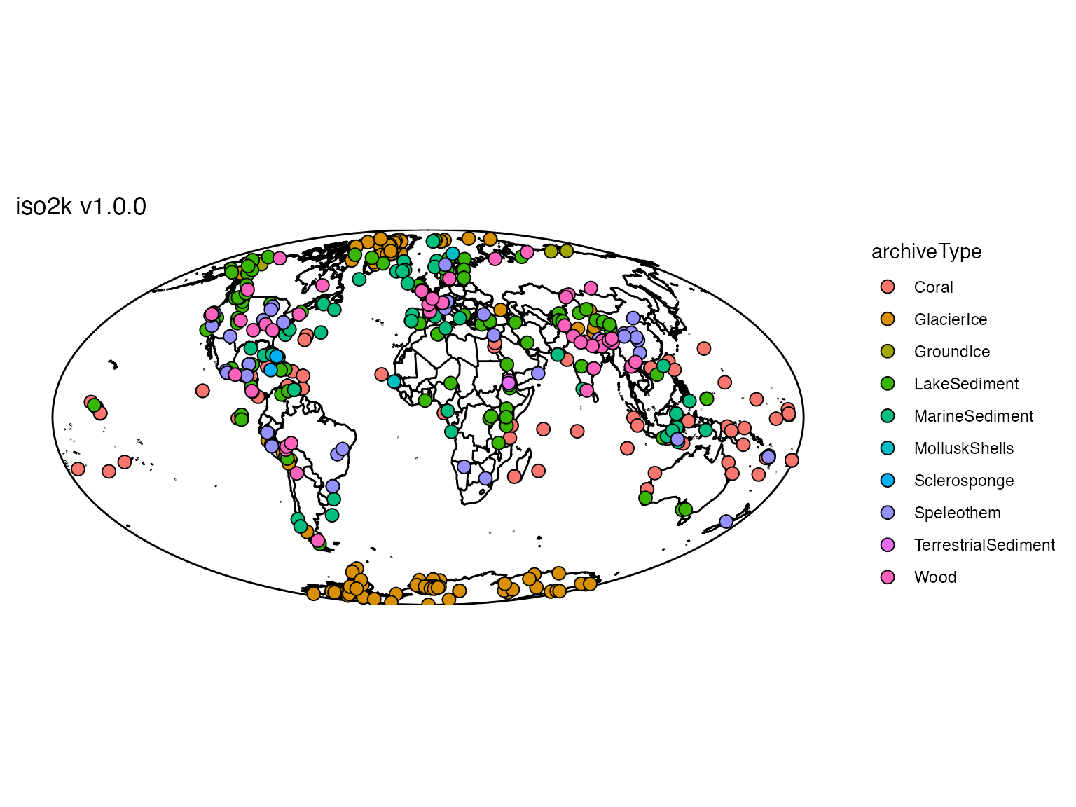
Now that the data are loaded, we can quickly map a bunch of LiPD files using mapLipd().

mapLipd(iso, global = TRUE,size = 3) + ggtitle("iso2k v1.0.0")

Now we’ve seen an overview of all the files we’ve loaded, but now we’d like to filter the data.

First, we’ll extract a TS object, the primary way to work with multiple LiPD files. A TS is a list object that has an entry for each, column, and is readily queryable.

TS <- extractTs(iso)

If you’re used to working in the tidyverse paradigm, you can also convert the TS object into a “tidyTs”, which is a large, long, tidy, tibble.

tTS <- tidyTs(TS,age.var = "year")

Now we’ll filter it based on a range of criteria.

iTS <- filter(tTS, paleoData_iso2kPrimaryTimeseries == TRUE,
              between(geo_latitude,66.5,90),
              between(year,1000,2000),
              paleoData_variableName == "d18O") %>% 
  arrange(geo_latitude)

OK, now we’ve filtered down to just Arctic $\delta^{18}O$ data during the past Millennium. We can use mapTs() to map the data coverage represented in iTS.

tm <- mapTs(iTS,
      projection = "stereographic",#for polar projections
      global = FALSE,
      color = "archiveType", #color by the archiveType
      shape = "paleoData_inferredMaterialGroup", #shape by the inferredMaterialGroup
      size = 4,
      bound.circ = TRUE
      )

print(tm)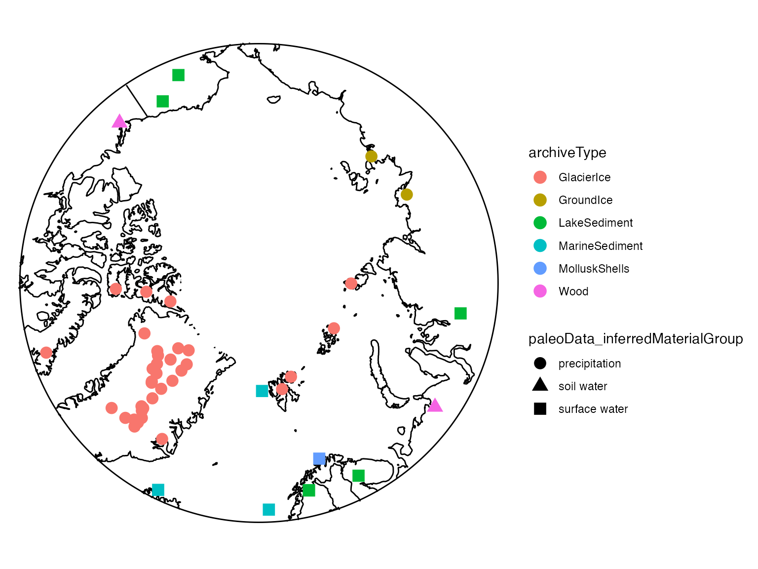

You can change the mapping options by passing options to basemap() which creates the base map. Try ?basemap for options.

Time availability

You can also quickly make a plot of availability through time.

plotTimeAvailabilityTs(iTS,age.range = c(1000,2000),age.var = "year",step = 20)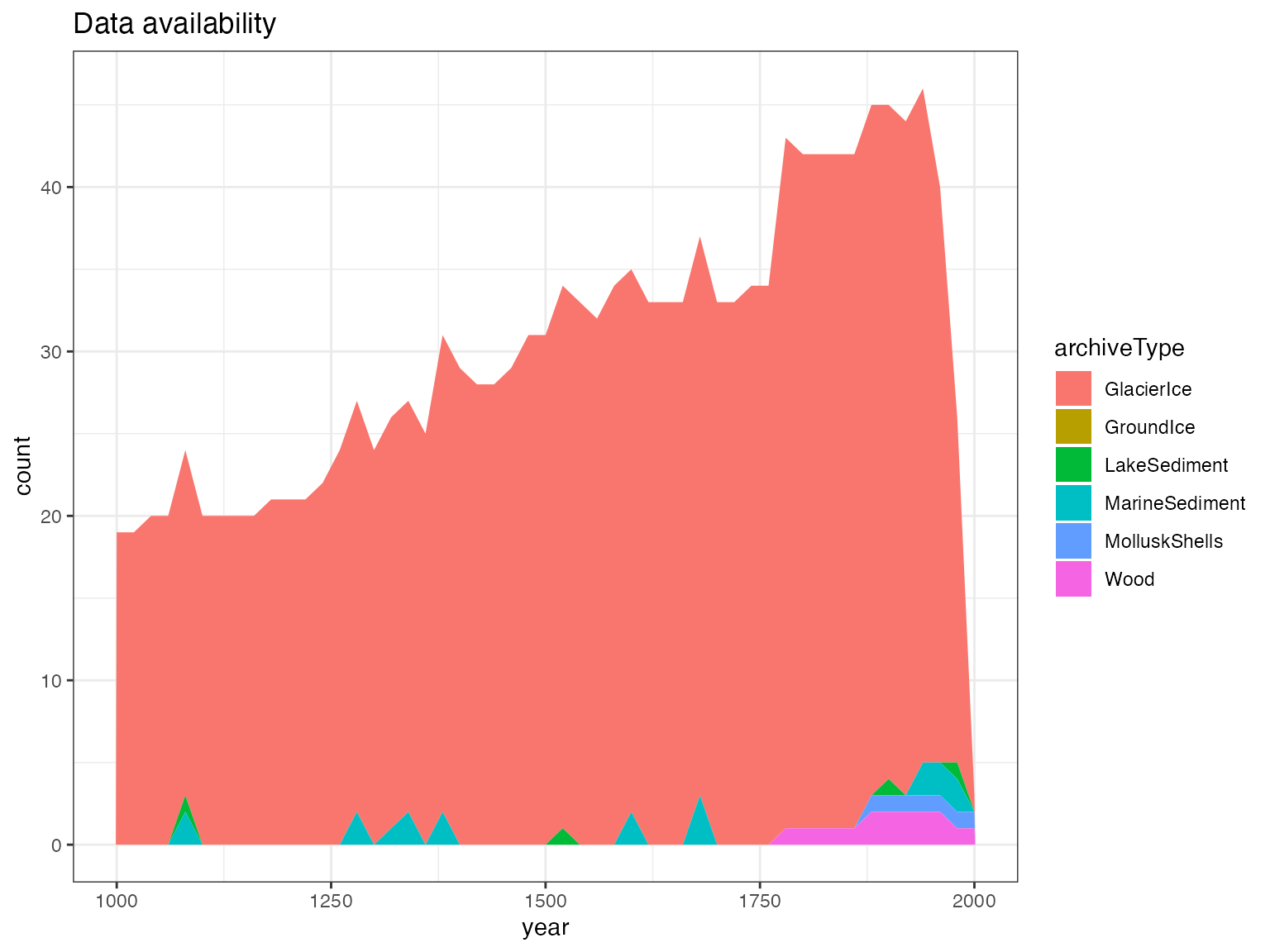

Plot a stack

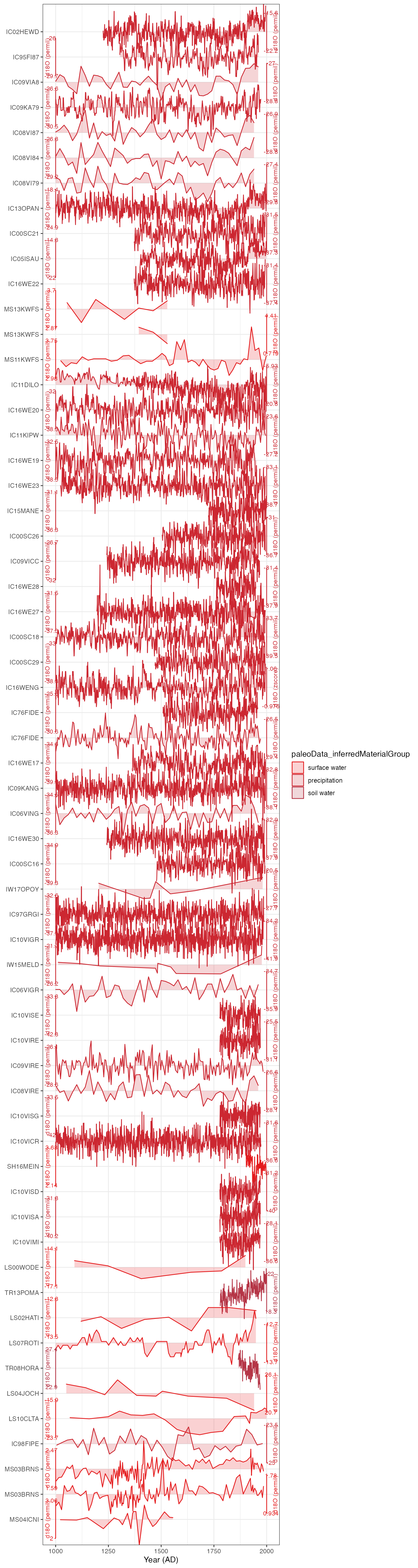
Finally, because we’re working with a “tidy” TS (a tibble), we can plot all the data using plotTimeseriesStack(). See the vignette on plotTimeseriesStack() for more details of how to use this function. Here we’ll plot all of these Arctic $\delta^{18}O$ datasets for the past millennium.

plotTimeseriesStack(iTS,color.var = "paleoData_inferredMaterialGroup",
                    color.ramp = function(nColors){RColorBrewer::brewer.pal(nColors,"Set1")}) 

Conclusion

Of course, now that the data are tidy, there’s a lot more you can do with these data using tidyverse tools.