Ensemble regression and calibration-in-time

Here, we replicate the analysis of Boldt et al. (2015), performing age-uncertain calibration-in-time on a chlorophyll reflectance record from northern Alaska, using geoChronR.

The challenge of age-uncertain calibration-in-time is that age uncertainty affects both the calibration model (the relation between the proxy data and instrumental data) and the reconstruction (the timing of events in the reconstruction). geoChronR simplifies handling these issues.

Let’s start by loading the packages we’ll need.

library(lipdR) #to read and write LiPD files
library(geoChronR) #of course
library(readr) #to load in the instrumental data we need
library(ggplot2) #for plotting

Load the LiPD file

OK, we’ll begin by loading in the Kurupa Lake record from Boldt et al., 2015. The system.file(...) part of this pulls the example file from the package directory. You’d like just enter the path as a string for typical use.

K <- lipdR::readLipd("http://lipdverse.org/geoChronR-examples/Kurupa.Boldt.2015.lpd")

## [1] "Loading 1 datasets from /var/folders/h1/8hndypj13nsbj5pn4xsnv1tm0000gn/T//RtmppYhGve/Kurupa.Boldt.2015.lpd..."
## [1] "reading: Kurupa.Boldt.2015.lpd"

Check out the contents

sp <- plotSummary(K,paleo.data.var = "RABD",summary.font.size = 6)

## [1] "Found it! Moving on..."
## [1] "Found it! Moving on..."
## [1] "Found it! Moving on..."
## [1] "Found it! Moving on..."
## [1] "Found it! Moving on..."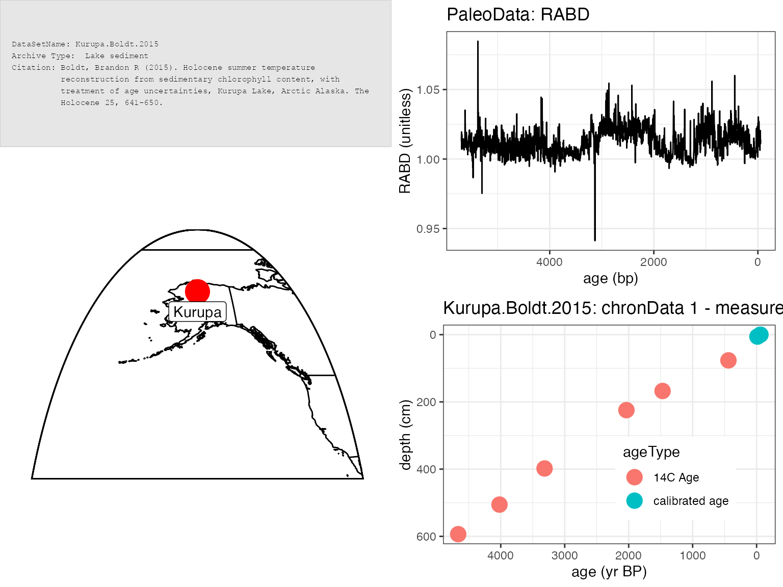

print(sp)

## TableGrob (4 x 4) "arrange": 4 grobs
##   z     cells    name                 grob
## 1 1 (1-1,1-2) arrange gTree[GRID.gTree.11]
## 2 2 (1-2,3-4) arrange       gtable[layout]
## 3 3 (2-4,1-2) arrange       gtable[layout]
## 4 4 (3-4,3-4) arrange       gtable[layout]

Create an age model with Bacon

K <- runBacon(K,
              lab.id.var = 'labID', 
              age.14c.var = 'age14C', 
              age.14c.uncertainty.var = 'age14CUncertainty',
              age.var = 'age', 
              age.uncertainty.var = 'ageUncertainty', 
              depth.var = 'depth', 
              reservoir.age.14c.var = NULL, 
              reservoir.age.14c.uncertainty.var = NULL, 
              rejected.ages.var = NULL,
              bacon.acc.mean = 10,
              bacon.thick = 7,
              ask = FALSE,
              bacon.dir = "~/Cores",
              suggest = FALSE,
              close.connection = FALSE)

##  Using a mix of cal BP and calibrated C-14 dates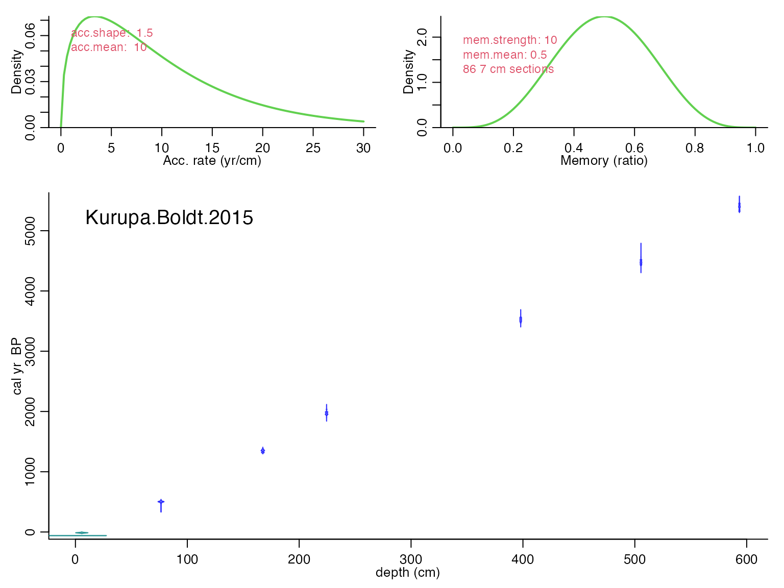

##  Run Kurupa.Boldt.2015 with 86 sections? (Y/n)

##  Will run 16,500,000 iterations and store 4,000

## Warning, this will take quite some time to calculate. I suggest increasing d.by to, e.g., 10

## Calculating age ranges...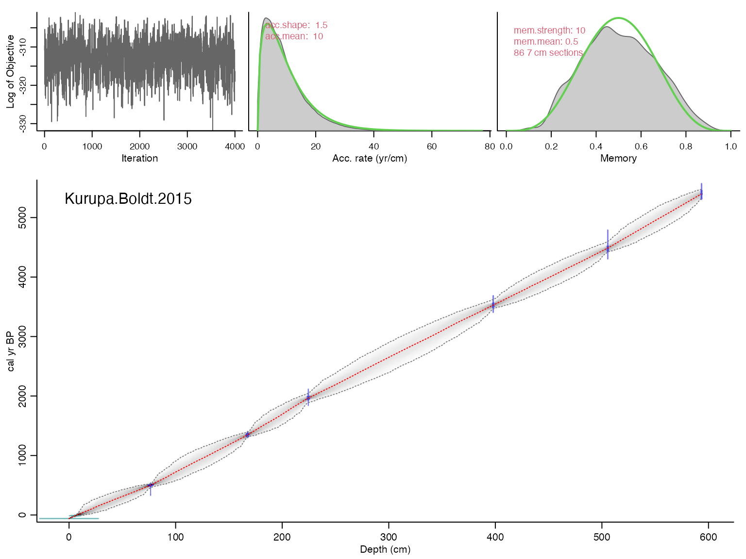

## 
## Preparing ghost graph...

## 
## Mean 95% confidence ranges 318 yr, min. 4 yr at 0 cm, max. 512 yr at 301 cm

## 100% of the dates overlap with the age-depth model (95% ranges)

##

## Warning, this will take quite some time to calculate. I suggest increasing d.by to, e.g., 10

And plot the ensemble output

plotChron(K,age.var = "ageEnsemble",dist.scale = 0.2)

## [1] "Found it! Moving on..."
## [1] "Found it! Moving on..."
## [1] "plotting your chron ensemble. This make take a few seconds..."

## Scale for x is already present.
## Adding another scale for x, which will replace the existing scale.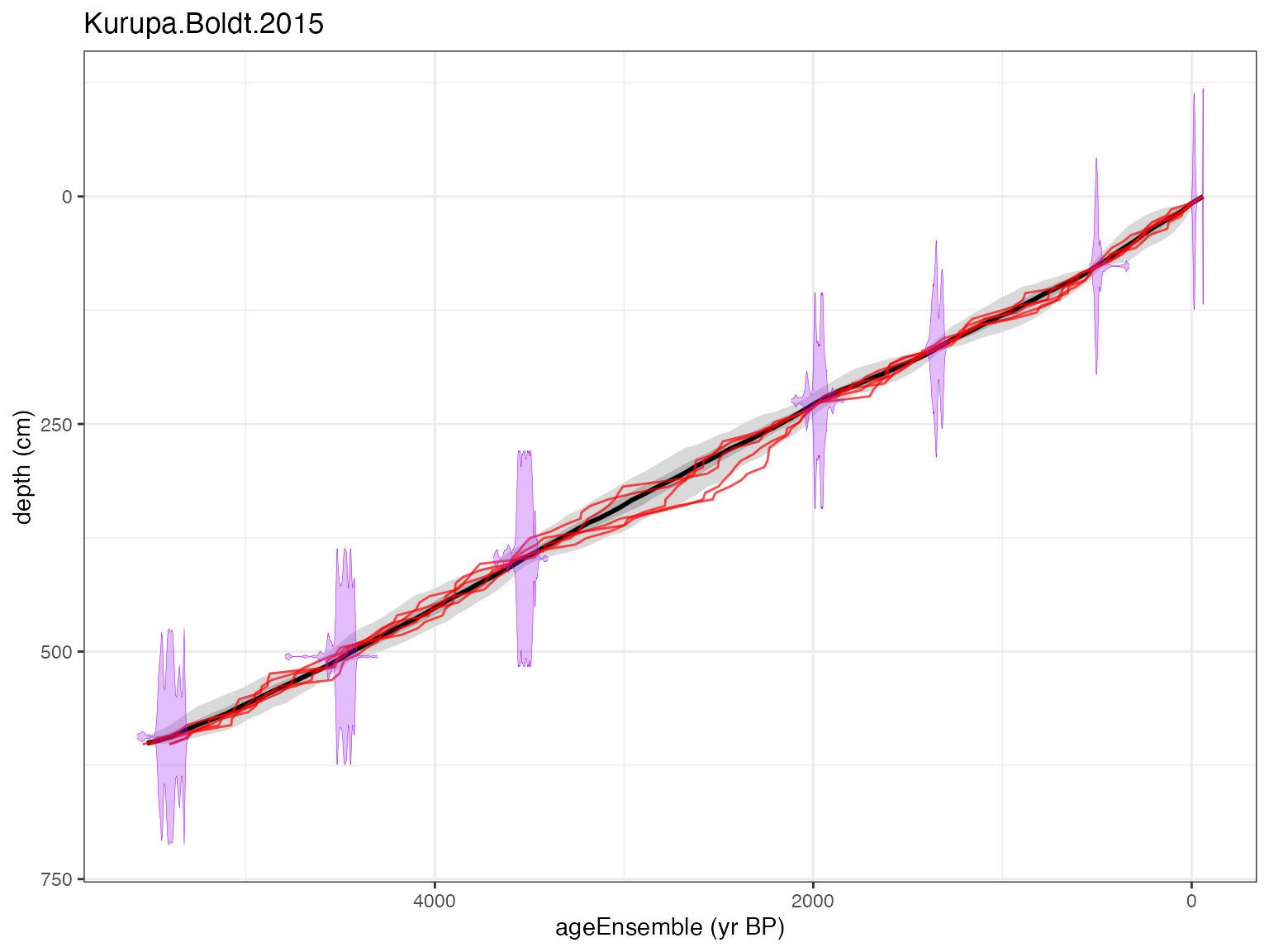

Map the age ensemble to the paleodata table

This is to get ensemble age estimates for each depth in the paleoData measurement table

K <- mapAgeEnsembleToPaleoData(K,age.var = "ageEnsemble")

## [1] "Kurupa.Boldt.2015"
## [1] "Looking for age ensemble...."
## [1] "Found it! Moving on..."
## [1] "Found it! Moving on..."
## [1] "getting depth from the paleodata table..."
## [1] "Found it! Moving on..."
## mapAgeEnsembleToPaleoData created new variable ageEnsemble in paleo 1 measurement table 1
## mapAgeEnsembleToPaleoData also created new variable ageMedian in paleo 1 measurement table 1

Select the paleodata age ensemble, and RABD data that we’d like to regress and calibrate

kae <-  selectData(K,"ageEnsemble")

## [1] "Found it! Moving on..."

rabd <- selectData(K,"RABD")

## [1] "Found it! Moving on..."

Now load in the instrumental data we want to correlate and regress agains

kurupa.instrumental <- readr::read_csv("http://lipdverse.org/geoChronR-examples/KurupaInstrumental.csv")

## Rows: 134 Columns: 2
## ── Column specification ────────────────────────────────────────────────────────
## Delimiter: ","
## dbl (2): Year (AD), JJAS Temperature (deg C)
## 
## ℹ Use `spec()` to retrieve the full column specification for this data.
## ℹ Specify the column types or set `show_col_types = FALSE` to quiet this message.

Check age/time units before proceeding

kae$units

## [1] "yr BP"

yep, we need to convert the units from BP to AD

kae <- convertBP2AD(kae)

Create a “variable list” for the instrumental data

kyear <- list()
kyear$values <- kurupa.instrumental[,1]
kyear$variableName <- "year"
kyear$units <- "AD"

kinst <- list()
kinst$values <- kurupa.instrumental[,2]
kinst$variableName <- "Temperature"
kinst$units <- "deg (C)"

Calculate an ensmeble correlation between the RABD and local summer temperature data

corout <- corEns(kae,rabd,kyear,kinst,bin.step=2,percentiles = c(.05,.5,.95 ))

And plot the output

Note that here we use the “Effective-N” significance option as we mimic the Boldt et al. (2015) paper.

plotCorEns(corout,significance.option = "eff-n")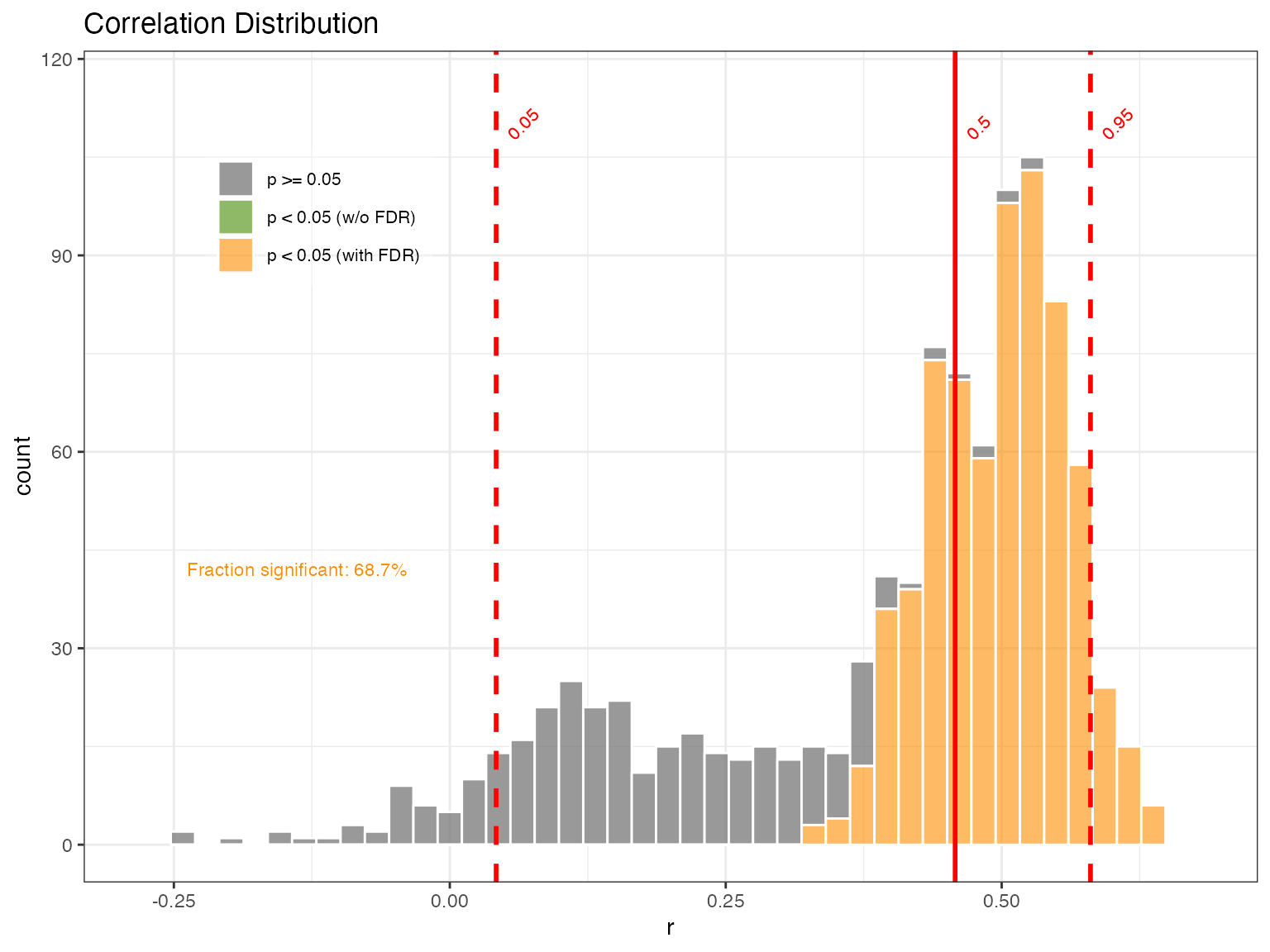

Mixed results. But encouraging enough to move forward.

Perform ensemble regression

OK, you’ve convinced yourself that you want to use RABD to model temperature back through time. We can do this simply (perhaps naively) with regession, and lets do it with age uncertainty, both in the building of the model, and the reconstructing

regout <- regressEns(time.x = kae,
                    values.x = rabd,
                    time.y =kyear,
                    values.y =kinst,
                    bin.step=3,
                    gaussianize = FALSE,
                    recon.bin.vec = seq(-4010,2010,by=20))

And plot the output

regPlots <- plotRegressEns(regout,alp = 0.01,font.size = 8)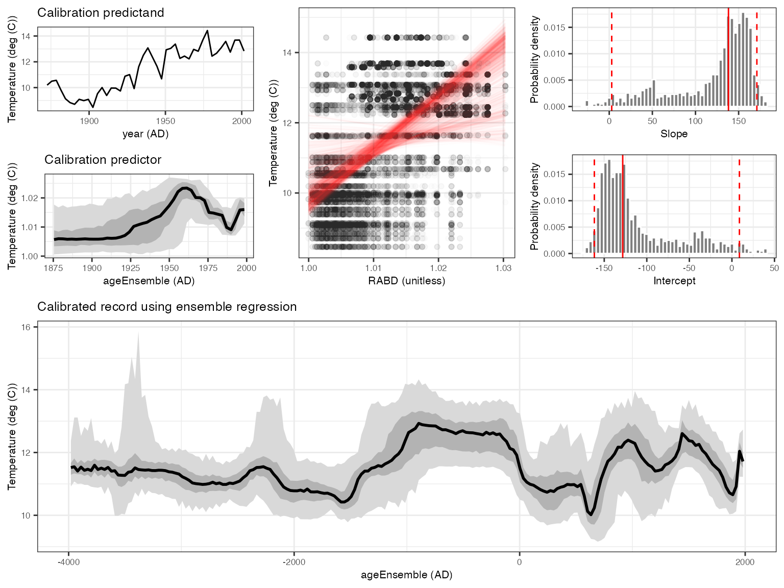

This result is consistent with that produced by Boldt et al., (2015), and was much simpler to produce with geoChronR.

In the next vignette learn about spectral analysis in geoChronR.

```

Ensemble regression and calibration-in-time

Nick McKay

2024-04-03