Plot a stack of proxy timeseries

Plotting a stack of proxy timeseries

A stalwart of paleoclimate data visualization, for good or bad, is stacking a bunch of timeseries vertically to examine similarities and differences. Although comparing timeseries in this way can be problematic, it remains a space-efficient way to visualize many records. It is straightforward to create such a plot with LiPD data in geoChronR.

Here we’ll load in a handful of data from PAGES2k v2.1.0 database, and explore some of these options.

Load the requisite libraries

We’ll be using a handful of libraries in this example

library(lipdR) #to read and interact with LiPD data
library(geoChronR) #for plotting mostly
library(magrittr) #we'll be using the magrittr pipe ( %>% ) for simplicity
library(dplyr) #and dplyr for data.frame manipulation
library(ggplot2) #for plotting

Load in your data

Load in some data. Below is an example of loading a zip file of LiPDs directly from the web. You can also load individual LiPD files from a url. You also might specify the path to a local file or folder here D <- readLipd("~/MyLipds/"), or use it interactive mode D <- readLipd(). If you’re selecting a directory in interactive mode, just click on any file in the directory that you want.

D <- readLipd("http://lipdverse.org/geoChronR-examples/euro/Euro2k.zip")

Extract those data into a timeseries object

OK, now you have a large list of all your files. It’s almost always to work with the data as a “timeseries object”, so let’s extract one of those.

TS <- extractTs(D)

Filtering the TS object for the data you want.

There will be two opportunities to filter your potentially very large collection of data down to what you want to analyze. Our next step, creating a “tidy” data frame, can be very slow with large TS options, so it’s best to filter what you can with the TS object first. See ?filterTs for options on how to do that. Here, we’re going to grab all the records with the “paleoData_useInGlobalTemperatureAnalysis” flag, and filter geographically a bit.

mts <- filterTs(TS, "paleoData_useInGlobalTemperatureAnalysis == TRUE") %>% 
  filterTs("geo_longitude > 0") %>% 
  filterTs("geo_latitude > 20")

Now create a “tidy” data.frame for querying, filtering and plotting.

The tidyTs() function will take a timeseries object and turn it into a long, “tidy”, data frame, where each row is an observation, and each column a variable. This will play very nicely with the tidyverse and facilitate efficient data analysis and visualzation. With large TS objects, this can result in data.frames with millions of rows, and can be quite slow to create.

tidyData <- tidyTs(mts,age.var = "year")

Now we can filter and structure our tidy data frame with just what we want using tidyverse tools

#filter for plotting
plot.df <- tidyData %>% 
  filter(between(year,1600,2000)) %>% #only years from 1600 to 2000
  filter(between(geo_longitude,0,50)) %>%  #only European longitudes
  filter(between(geo_latitude,20,60)) %>%  #between 20 and 60 N
  filter(interpretation1_variable == "T") %>% #only variables sensitive temperature
  group_by(paleoData_TSid) %>% #group by column
  arrange(archiveType) #and sort by archiveType

That last arrange() command controls the order of the data frame, and will also control the order of the stack.

OK, we have a tidy data.frame that includes the data we want to plot.

The key function for this is plotTimeseriesStack(), and has many options (?plotTimeseriesStack). We can start simply by giving it the data frame and using the default options:

#plot the stack and color by Archive type
plotTimeseriesStack(plot.df)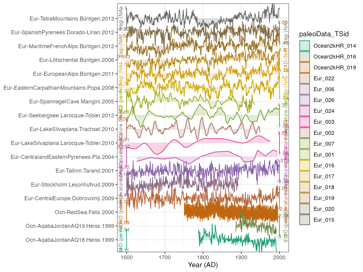

## Adjusting the options

OK! We have a plot! It looks decent, and by default it colors it by the TSid, but we might rather color it by archiveType. We do that simply:

plotTimeseriesStack(plot.df,color.var =  "archiveType")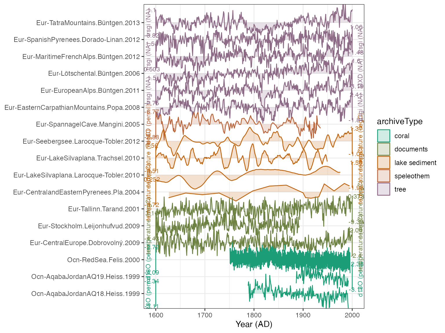

Better. But we need to make the axis labels smaller, and want to give it some more intuitive colors for each archive

plotTimeseriesStack(plot.df,
                    color.var =  "archiveType",
                    lab.size = 2,
                    color.ramp = c("coral","black","blue","magenta","dark green"))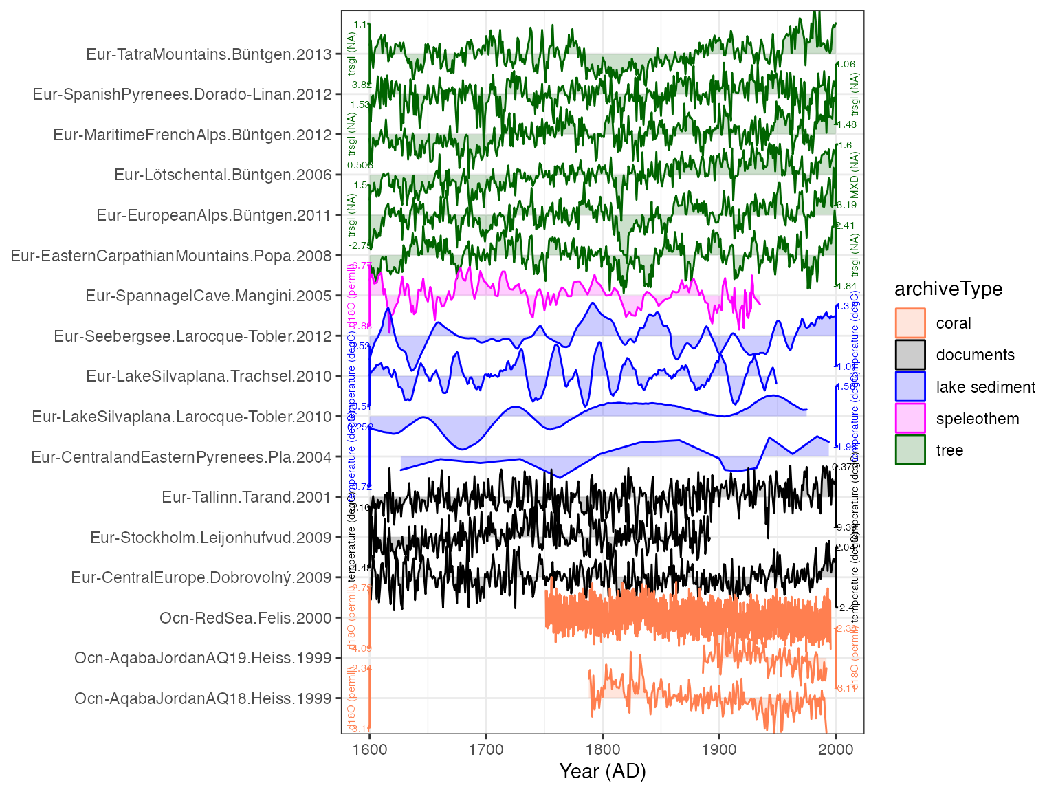

That looks pretty good! Perhaps we think this is too colorful for a journal submission, and we don’t want the shading along each line. And we also want to arrange the lines by latitude instead of archive.

plot.df <- arrange(plot.df,geo_latitude) #order by latitude
                   
myPlot <- plotTimeseriesStack(plot.df, #create another plot, storing the output
                    lab.size = 2,
                    color.ramp = "black",#if we specify one color, all the records will get that
                    fill.alpha = 0, #make the fill transparent
                    lab.space = 3, #add it a bit more space between the axis labels and ticks
                    line.size = 0.4) #make the lines a bit thinner
print(myPlot)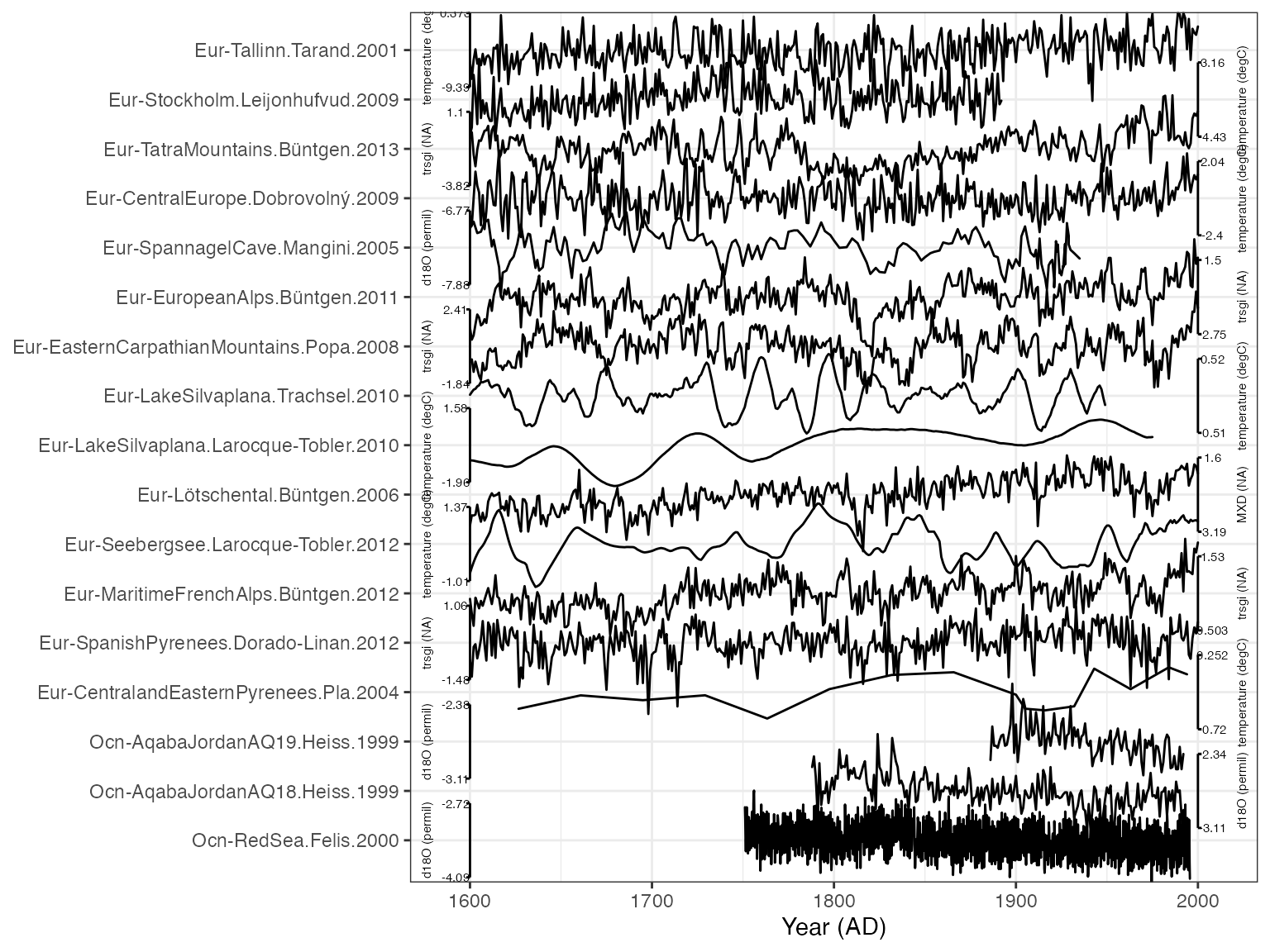

Additional manipulation of the plot with ggplot2

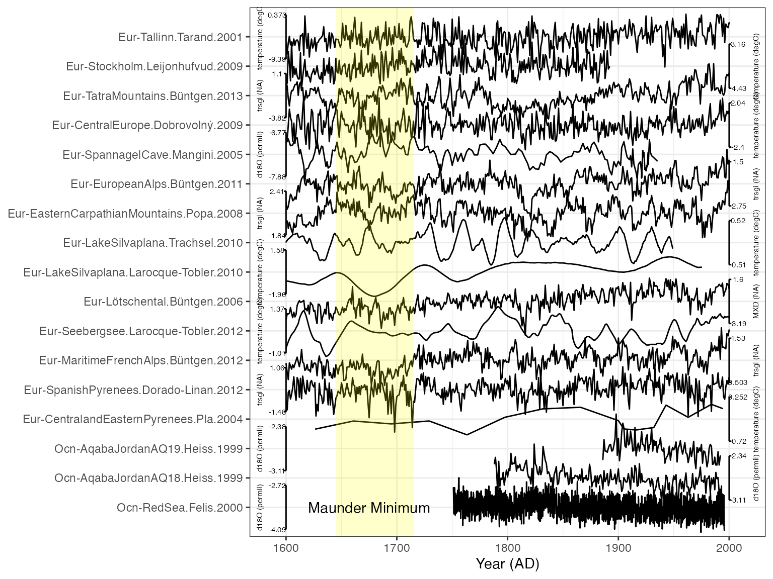
The output of plotTimeseriesStack is a standard ggplot object, which means you can customize and adjust axes and add additional layers. As an example, let’s add rectangular box to highlight an interval of interest, the Maunder Minimum.

The x-axis for our plot is time, and the y-axis is the number of records, counting from the bottom.

myPlot + annotate(geom = "rect", colour = NA, fill = "yellow", xmin = 1645, xmax = 1715, ymin = 0, ymax = length(unique(plot.df$dataSetName))+1,alpha = 0.2) +
  annotate(geom = "text", x = 1675, y = 1, label = "Maunder Minimum")

Conclusion

plotTimeseriesStack() is handy for quick visualization, but also can be tinkered to near-publication-quality. For now, this does not work with ageEnsembles, although we hope to include this in the future.

Nick McKay

2024-09-11